Help
Select desired topic to show help
Power losses
For all available TDK power materials, the power loss per volume and per mass can be represented as a function of the temperature T, the frequency f and the flux density B. The number of measurement data available in the program exceeds the number of data specified in the data book by far. It is possible to display only one curve in one chart.
Procedure:- Select desired parameter: power losses versus temperature, frequency, flux density or performance factor.
- Select desired material.
- Define the parameters that are to be presented on vertical axe.
- Click on button "OK"
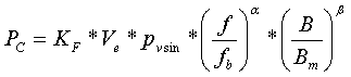
- f (kHz) is the actual operating frequency and B (mT) the actual operating peak sinusoidal flux density at an operating temperature Top(°C)
- pvsin is the loss density in kW/m3 at temperature Top(°C), frequency fb (kHz) and peak sinusoidal flux density Bm (mT)
- Ve (mm3) is the magnetic volume of the core
- α is the Steinmetz exponent for frequency and β the Steinmetz exponent for flux density for the ferrite material at Top
- pvsin is measured on standard ring cores
- KF is a multiplication factor for the particular core shape in use
- These coefficients you can simply copy to clipoard
Complex permeability
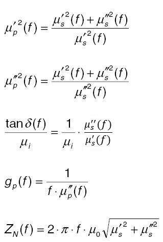
For all available TDK materials, the complex permeability can be represented as a function of the frequency. You can select one of seven display types μs’ (f), μs’’ (f), μp’ (f), μp’’ (f), gp(f), tanδ/μi(f) or Z_N(f). The different parameters provide an optimum material comparison for various applications:
- the relative loss factor tanδ/μ for filter's inductors with high Q
- the parallel conductance gp(f), which is directly proportional to the insertion loss, for broadband transformers
- the normalized impedance Z_N(f) for EMI suppressors
- The relationship among the different parameters is given as follows:
- Select the desired material.
- Select whether μs’ (f), μs’’ (f), μp’ (f), μp’’ (f), gp(f), tanδ/μi (f) or Z_N(f) are to be represented. The graph will be displayed.
Effective permeability µe vs. T
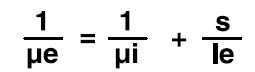
For all available TDK materials, the core-form-specific μe(T) characteristics based on the μi(T) material curve (measured on ring cores) can be calculated. This calculation is performed according to the well-known equation:
- Select the desired core.
- Specify the core form (optionally: low profile, with hole). Note: Please observe that not all combinations are valid (e.g. in low profile, only RM cores are available). Values will not be output if an invalid combination was specified.
- Select the desired material.
- Select the type of representation μe(T) or (μe(T) - μe(T1))/μe(T).
- Enter the desired air gap in the s field.
- Click on button "OK" to shot the effective permeability as a function of the temperature.
P trans (Transferable Power)
For all power materials and most cores, the transferable power Ptrans can be determined.
Procedure:- Click on the Core Form button in the main window. The Core data window will be opened.
- Select Ptrans.
- Select the desired core.
- Specify the core form. Note: Please observe that not all combinations are valid. Values will not be output if an invalid combination was specified.
- Select the desired material.
- Correct for the default thermal resistance Rth value (free-air convection), if a better figure is known for your application.
- Enter the desired values in the dTCu, dTFe and f input fields.
- Correct for the default copper space factor fCu=0.4 if a better figure is known for your application.
- If a wire calculation on the selected core type has been performed previously, click the “get Rac/Rdc” button to consider proximity and skin effects in the Ptrans calculation.
- Select the appropriate converter type in the pull down menu.
- Ptrans will be displayed in the output field after pressing the “Calculate” button.
Further description of the input fields:
fCu: copper space factor
dTCu: copper temperature rise [K]
dTFe: ferrite temperature rise [K]
The transferable power Ptrans of transformers can be calculated by the following approximation:

The constant C relates to the operation mode which is:
C = 1 in push-pull converters
C = 0,71 in single-ended converters
C = 0,62 in flyback converters (1)
Further quantities in equation (1) are the switching frequency f,
the sweep of flux density ΔB, the current density S,
the winding cross section An and the effective area Ae.
DC-BIAS
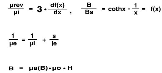
For all available TDK power materials and most core shapes, the reversible permeability can be calculated as a function of the DC-current as well as of the DC-field with a given Al value. For this purpose, the temperatures T = 25 °C and T = 100 °C are taken into consideration. With a given number of turns, the reversible inductance and the magnetic energy can additionally be calculated.
Procedure:- Select the desired core.
- Specify the core form. Note: Please observe that not all combinations are valid. Values will not be output if an invalid combination was specified.
- Select the desired material.
- Select the desired temperature (T = 25 °C or T = 100 °C).
- Select the measurands that are to be represented on the X- and Y-axes.
- Enter the desired values for the unbiased inductance L in [mH], the DC-current Idc in [A] and the roll-off d in[%] in the corresponding input fields.
- Click the yellow “Calculate” button. The calculated values will be displayed in the output fields and a corresponding plot shown.
- If you want to change the Al value and/or number of turns N for new plot data, enter the new values and click on "Calculate" button.
The new resulting unbiased inductance and the graph will be displayed.
Underlying formulae:
Third harmonic distortion
For a given core and a given material, the calculated ratio of the AC-to DC-resistance vs. Frequency for sinusoidal current waveforms can be displayed.
Procedure:- Select the desired core.
- Specify the core form. Note: Please observe that not all combinations are valid. Values will not be output if an invalid combination was specified.
- Select the desired material.
- Select the desired input option: turns ratio/inductance/resistances or AL-value/number of turns/wire diameter.
- Enter the desired values in the corresponding input fields. The calculated values will be displayed in the output fields.
Underlying Formulae:
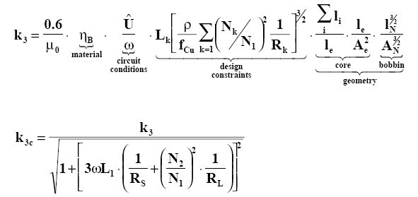
By using the following equations the third harmonic distortion
k3 for the voltage based on Rayleigh´s hysteresis model can
be calculated. The in-circuit distortion k3c follows form
consideration of the impedance conditions. 1)
Wire calculation
For a given core and a given material, the calculated ratio of the AC-to DC-resistance vs. Frequency for sinusoidal current waveforms can be displayed.
Procedure:- Select the desired core.
- Specify the core form. Note: Please observe that not all combinations are valid. Values will not be output if an invalid combination was specified.
- Select the total number of turns
- Select the number of layers
- Click on the button “Calculate”
- All mandatory fields are marked with star
- The graph will be displayed. If the window fill factor fw surpasses 100% a warning message will be shown.
Procedure:
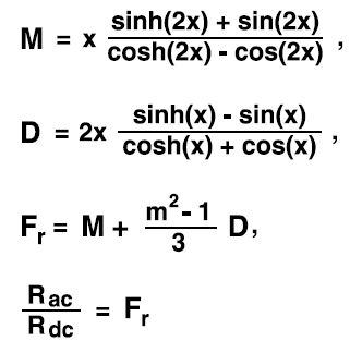
By using the following equations the winding copper losses
for sinusoidal current can be estimated. 1) . x stands for
the ratio of the wire diameter to the frequency-dependent
penetration depth, m stands for number of layers.
Non-sinusoidal core loss density - introduction
The performance of any power ferrite core material depends primarily on the amplitude and nature of time-variation of the magnetic flux density impressed upon it at the operating temperature. The time-variation of magnetic flux density includes the time-period of repetitive variation and the waveform of variation. In general the nature of variation of magnetic flux is not sinusoidal for practical Switch Mode Power Supply (SMPS) circuits. Manufactures of power ferrite materials provide extensive measured data on core losses with sinusoidal flux. A numerical model together with a user-friendly nomogram to compute core loss with non-sinusoidal flux from the measured data with sinusoidal flux is presented to provide design help for power ferrite material selection taking into account the actual flux waveform of the user.
The concept of equivalent sinusoidal frequency
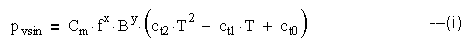
The expression for core loss density pvsin for a power ferrite material for a sinusoidal flux density amplitude B, at frequency f and operating temperature T is given as:

This is the basic Steinmetz equation and Cm, ct2, ct1 and ct0 are constants for a particular power ferrite material and are usually defined for specific ranges of frequency, flux density and temperature. M.Albach, Th. Durbaum and A.Brockmeyer <11> have extended this to non-sinusoidal flux densities by introducing the concept of an equivalent sinusoidal frequency fsineq.
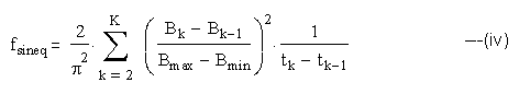
The frequency of the non-sinusoidal flux waveform is f, amplitude is B and the equivalent sinusoidal flux waveform has peak amplitude equal to that of the non-sinusoidal waveform. The equivalent sinusoidal frequency is given by:
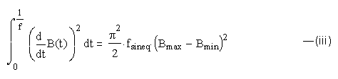
The periodic non-sinusoidal flux density is given as B(t), the maximum and minimum values of flux density in a cycle are Bmax and Bmin respectively. B(t) is assumed to have unique maxima and minima in a cycle to avoid creation of sub-loops of magnetization. For piece-wise linear flux waveforms with K-1 linear segments (K points) the integral (iii) is replaced by the summation:
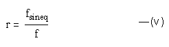
Defining a variable r as:
From (i), (ii) and (v):
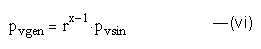
The basic circuits, flux density waveforms and an approximate equivalent sinusoid are shown for few typical SMPS topologies (the actual flux density curves are shown in bold lines and the equivalent sinusoid in dotted lines in all the cases with time t and flux density B(t) as axes) in Figs 1 to 12. For the converter topologies listed the analytical expression for r as a function of duty-cycle has been found and plotted using either the integral (iii) or the summation (iv). The flux waveforms may be referenced to Cyril W. Lander <12> or any other text on Power Electronics. The power loss density pvgen may be computed for a given converter using the analytical expressions for r and the value of Steinmetz frequency exponent x for the ferrite material using expression (vi) above. The power loss density pvsin in (vi) can be obtained from measured data of the ferrite material at sinusoidal frequency at the desired operating temperature and choosing the amplitude of flux density so as to have the same peak excursion as the desired waveform. All the flux waveforms listed have single maxima and minima in a cycle so that there are no multiple magnetizing loops in a cycle.
Pushpull converters
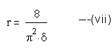
From (iv), K=6, duty cycle 0<δ<=1 and in both the cases
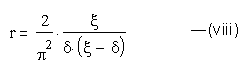
Fly back converter with discontinuous current
From (iv), K=4; the duty-cycle δ and the extinction-cycle ξ are related by:
0<δ<ξ=<1
r is given by:
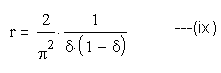
Flyback converter with continuous current
From (iv), K=3; the duty-cycle
0<δ<1
Zero-Current-Switch (ZCS) Resonant Converter
From (iii) the equivalent sinusoidal frequency feqsin,
the resonant frequency fr,
and the duty-cycle δ, 0<δ<1 are related by:
2 * fr = feqsin = f / δ
hence
r = 1 / δ ---(x)
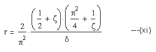
Zero-Voltage-Switch (ZVS) Resonant Converter
The resonance frequency is fr, half-period of resonance is
1 / (2 * fr), the charge recovery time of the inductor is tr,
a variable ζ is defined as
ζ = tr * fr.
From (iii), fr, ζ, and the duty-cycle δ, 0<δ<1
are related by:
δ = f * (ζ + 1/2) / fr
The general expression for r is given as:
An optimum value of ζ may be found by differentiating (xi):
This yields a minimum value of r:
rmin = 0.903 / δ (xii)
The corresponding resonant frequency is
fr = 0.95 * f / δ
The variation of r with δ for the different topologies is shown in Figs. 11 &12.
The value of r increases with reducing duty-cycle for pushpull, ZCS and ZVS.
For flyback the value of r increases at asymmetrical duty-cycles.
Duty-cycle
The influence of duty-cycle on converter efficiency and choice of operating temperature
For sinusoidal flux N95 is a more efficient choice than N97 up to an operating temperature of 90°C (Fig.25). For a pushpull converter operating at 50% duty-cycle N95 remains more efficient than N97 up to a temperature of 80°C.
An user friendly nomogram has been developed which accepts the following inputs:
- TDK power material : N49 / N87 / N92 / N95 / N97
- Converter type : sine / pushpull / continuous current flyback / discontinuous current flyback / ZCS / ZVS
- Operating frequency f : 25 / 50 / 100 / 200 / 300 / 500 / 700 / 1000 kHz
- Flux density amplitude B : 25 / 50 / 100 / 141 / 200 / 300 mT
- Operating temperature T : 25 / 40 / 60 / 80 / 100 / 120 °C
- Duty-cycle δ: as applicable.
The Steinmetz exponents ‘x’ and ‘y’ for the TDK materials are built-in. The nomogram outputs the following parameters for the above inputs:
- The ratio of equivalent sinusoidal frequency to operating frequency : r
- The ratio of core loss density for the selected case to equivalent sinusoidal : rx-1
- The core loss density pvgen for the selected case in kW/m3
- For an x-axis selection of f / B / T the nomogram outputs the curve of pvgen for the other selected parameters.
- For the selection of the material, the converter type, f / B / T the nomogram outputs the graph of rx-1 (the ratio of core loss under given condition to sinusoidal core loss at f / B / T for the same material) versus applicable duty-cycle.
Impedance Z
Ring cores to suppress line interference
With the ever-increasing use of electrical and electronic equipment, it becomes increasingly important to be able to ensure that all facilities will operate simultaneously in the context of electromagnetic compatibility (EMC) without interfering with each others’ respective functions. The EMC legislation which came into force at the beginning of 1996 applies to all electrical and electronic products marketed in the EU, both new and existing ones. So the latter may have to be modified so that they are neither susceptible to electromagnetic interference, nor emit spurious radiation. Ferrite cores are ideally suited for this purpose since they are able to suppress interference over a wide frequency range.
At frequencies above 1 MHz, ferrite rings slipped over a conductor lead to an increase in the impedance of this conductor. The real component of this impedance absorbs the interference energy.
A ferrite material's suitability for suppressing interference within a specific frequency spectrum depends on its magnetic properties, which vary with frequency. Before the right material can be selected, the impedance lZl must be known as a function of frequency. The curve of impedance as a function of frequency is characterized by the sharp increase in loss at resonance frequency.
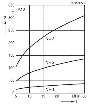
Measurement results
The measurements shown here were made at room temperature (25 ±2) °C using an HP 4191A RF impedance analyzer with a flux density of B ≤ 1 mT.
The maximum of the impedance curve shifts to lower frequencies as the number of turns increases; this is due to the capacitive effect of the turns (see figure, using R 25/15 as an example).
The impedance curves of different materials are summarized for direct comparison. The normalized impedance |Z|n = |Z| / N2 * (le /Ae) were used to display material properties only. The geometry factor was calculated on the basis of the core dimensions.
These normalized impedance curves are guide values, mostly measured using toroidal core R10 with a number of turns N = 1 (wire diameter 0.7 mm); they may vary slightly, depending on the geometry.
Reference List
[1] E. C. Snelling [1988], Soft Ferrites, Butterworths, 2nd Edn.
[2] P. L. Dowell [1966], Effects of eddy currents in transformer
windings, Proc. IEE, Vol. 113, No. 8.
[3] B. Carstens [1995], Calculating Skin and proximity effect
conductor losses in switch mode magnetics, PCIM’95 seminar notes.
[4] T. Werner, J. Hess [1996], Core loss measurements in
high frequency power materials-measurement methods for the
frequency range up to 10 MHz, Proceedings of the PCIM’96, pg. 611-622.
[5] R. Gaus [1911], Die Gleichung der Kurve der reversiblen
Suszeptibilität, Phys. Z. 12, pp 1053 - 1054
[6] W. Kampczyk, E. Röß [1978], Ferritkerne, Siemens AG
[7] G. Roespel [1978], Effect of the magnetic material on the
shape and dimensions of transformers and chokes in switched-mode
power supplies, Siemens AG München, J. of Magn. and Magn.
Materials 9, pp 145 - 149
[8] M. Esguerra [1997] , “Ferrite Core Design for Broadband
Design of Telecom Transformers”, MMPA User´s Conference, Chicago.
[9] H. Meuche, M. Esguerra [1999] , “Ferrite Cores for xDSL:
Optimum Selection”EMCW´99, Cincinatti.
[10] P.Mukherjee : Core losses in power ferrite materials
with non-sinusoidal flux
[11] M.Albach, Th.Durbaum and A.Brockmeyer, 27th Annual IEEE
power Electronics Specialists Conference, 1996, Italy, pp 1463-1468
[12] Cyril W. Lander, Power Electronics, McGraw Hill Book Company, pp 274-276